How To Highlight Missing Values In Excel

09 Oct, 2021

This video demonstrates how to highlight cells with missing values in Excel. Get excel example file.

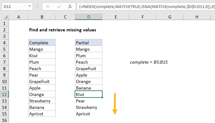
Excel Formula Find And Retrieve Missing Values Exceljet

Values that are missing.

How to highlight missing values in excel. The IF function returns the confirmation using the values Is there Missing. Automatically Highlight Active Row in Excel Life Hacks 365. Compare two columns for highlighting missing values with Kutools for Excel.

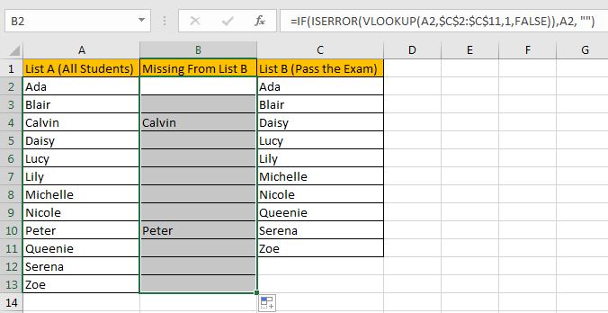
Cell B3 is highlighted the value is not found in the other list. In this tutorial we will help you to find out missing values via two ways the first one is by Conditional Formatting function in excel the second one is by using formula with VLOOKUP function. In the box next to values with pick the formatting you want to apply to.

Click on cell A2 and press Ctrl-Alt-V and then select the Paste Values option and press OK 6. Excel cant highlight duplicates in the Values area of a PivotTable report. 1 In the Find Values in box specify the range of Fruit List 1.

With conditional formatting its important to enter the formula relative to the active cell in the selection which is assumed to be A1 in this case. Conditional formatting is used to highlight cells with missing values and to cou. Now if the COUNTIF function returns 0 zero that means that the value is not found in the other cell range and the logical expression returns TRUE.

Next select Duplicate values. Select the cells you want to check for duplicates. For example to highlight values A1A10 that dont exist C1C10 select A1A10 and create a conditional formatting rule based on this formula.

Then select Highlight Cells Rules. Highlight values that are equal to 15. COUNTIF C1C10 A1 0 Note.

The formula will be Row a1HighlightRow where HighlightRow is the name of the defined range in Step 1Then click the format button. In the Compare Ranges dialog box you need to. In the example shown the formula in G6 is.

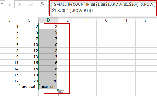
Use of COUNTIF and IF function. Add an Up arrow icon to cell values above 10. Function MissingSequence Rng As Range As String Dim iCnt As Integer For iCnt 65 To 90 ASCI characters for alphabet A-Z Dim iNum As Integer For iNum 100 To 999 Dim sCheck As String sCheck Chr iCnt iNum If RngFind sCheck lookatxlWhole Is Nothing Then Dim sMissingNumbers As String sMissingNumbers sMissingNumbers sCheck End If Next Next.

You can use behavior directly inside an IF statement to mark values that have a zero count ie. For example to highlight values A1A10 that dont exist C1C10 select A1A10 and create a conditional formatting rule based on this formula. Get an official version of MS Excel from the following link.

Excel also allows you to. You can use the below formula to highlight the missing values in Excel. Apply an italic bold font style if the value is between 70 and 90.

Apply a green font color if the text contains Montana. Highlight missing values Jump To. The generic formula for finding the missing values using the MATCH function is written below.

With conditional formatting its important to enter the formula relative to the active cell in. Highlight range E1E500 and press the Delete key to erase column E Charles. Firstly the lookup value is searched in the particular column of the table array.

This check can be passed as the logical test to the IF statement which will update the status of the entry accordingly. Then the matched values will give us the confirmation using the IF function. Apply a yellow fill to duplicate values.

In the format cells window switch to the fill tab and choose the color you want to use as the color to highlight the active row. A Duplicate Values settings box will open where you can define the formatting and select between Duplicate or Unique values. Select cells in List A where you want to highlight the values not in List B.

Click Home Conditional Formatting Highlight Cells Rules Duplicate Values. MATCH will look for the position of a certain item and will generate a NA error if the value is not found. Click the Kutools Select Select Same Different Cells to open the Compare Ranges dialog box.

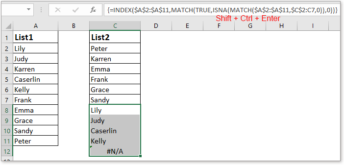
Missing values can also be found with the help of MATCH function. And then click Home Conditional Formatting New Rule see screenshot. IFCOUNTIF list F6 OKMissing where list is a named range that corresponds to the range B6B11.

From the Home tab select the Conditional Formatting drop down.

Group Data In An Excel Pivottable Pivot Table Excel Data

Excel Formula Sum Time With Sumifs Excel Formula Sum Getting Things Done

Compare Two Columns And Add Missing Values In Excel

How To Compare Two Columns To Find Missing Value Unique Value In Excel Free Excel Tutorial

Last Year Microsoft Announced The Introduction Of A New Group Of Functions In Excel Known As Dynamic Array Functions One Of These T Excel Filters Function

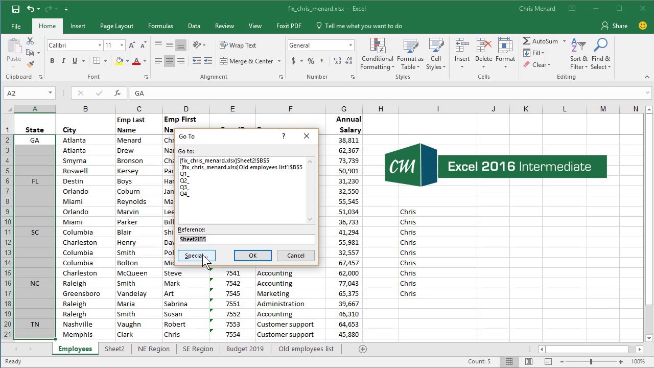
Ctrl Enter To Fix Missing Data In Excel By Chris Menard Youtube

Remove Formulas In Excel Excel Shortcuts Excel Tutorials Microsoft Excel

How To Identify Missing Numbers Sequence In Excel

How To Highlight Blank Values In Excel With Or Formula In 2020 Excel Tutorials Excel Formula Ex Excel Tutorials Microsoft Excel Tutorial Excel Formula